Getting started with JAGS for Bayesian Modelling
In the past if you wanted to do some Bayesian Modelling using a Gibbs sampler you had to rely on Winbugs but it isn’t open source and it only runs in Windows. The JAGS project started as a full feature alternative for the Linux platform. Here are some instructions for getting started
First install the required dependencies. In my Ubuntu 11.04, is something like:
sudo apt-get install gfortran liblapack-dev libltdl-dev r-base-coreFor Ubuntu 11.04 you have to install JAGS from sources, but it seems that this version will be packaged in the next Ubuntu release. Download the software from here and install.
tar xvfz JAGS-3.1.0.tar.gz
cd JAGS-3.1.0
./configure
make
sudo make install
Now fire R and install the interface package rjags
$ R
...
> install.packages("rjags",dependencies=TRUE)
Now let’s do something interesting (although pretty simple). Let’s assume we have a stream of 1s and 0s with an unknown proportion of each one. From R we can generate such distribution with the command
> points <- floor(runif(1000)+.4)that generates a distribution with roughly 40% of 1s and 60% of 0s. So, our stream consists of a sequence of 0s and 1s generated using the uniform(phi) distribution where the phi parameter equals 0.4.
If we don’t know this parameter and we try to learn it, we can assume that this parameter has prior uniform in the range [0,1] and thus the model that describes this scenario in the Winbugs language is
model
{
    phi ~ dunif(0,1);
    y ~ dbin(phi,N);
}
In this model N and y are known, so we provide this information in order to estimate our unknown parameter phi. We create the model and query the resulting parameter distribution:
> result <- list(y=sum(points), N=1000)
> result
$y
[1] 393

$N
[1] 1000

> library(rjags)
Loading required package: coda
Loading required package: lattice
linking to JAGS 3.1.0
module basemod loaded
module bugs loaded
> myModel <- jags.model("model.dat", result)
Compiling model graph
   Resolving undeclared variables
   Allocating nodes
   Graph Size: 5

Initializing model

> update(myModel, 1000)
  |**************************************************| 100%
> x <- jags.samples(myModel, c('phi'), 1000)
  |**************************************************| 100%
> x
$phi
mcarray:
[1] 0.3932681

Marginalizing over: iteration(1000),chain(1)

>
So the inferred value of phi is 0.3932. One interesting thing in Bayesian statistics is that it does not estimate points, but probabilistic distributions over the parameters. We can see how the phi parameter was estimated by examining the Monte Carlo Chain and the distribution of the generated values during the simulation
> chain <- as.mcmc.list(x$phi)
> plot(chain)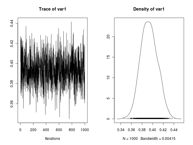
Where we can see that the values for phi in the chain were centered around the 0.4, the true parameter value.